VaR Revisited

• VaR is defined as the maximum dollar (or percentage) amount expected to be lost over a given time horizon, at a pre-defined confidence level. For example, if the 95% one-month VAR is $1 million, there is 95% confidence that over the next month the portfolio will not lose more than $1 million.

Arithmetic and Geometric Returns

• ARITHMETIC RETURNS : 
• GEOMETRIC RETURNS : 

Calculation of VaR using Historical Simulation

• Method :
• 1. The return observations are sorted in any manner.
  2. The required VaR corresponding to the confidence level (or significance level) is located. If α is the level of significance, and n is the total number of observations, then the corresponding VaR would be the  α×n+1^th lowest observation.

Estimating Parametric VaR

• Normal VaR 
  • α %  VaR is given by –
  • -μ_{P/ L}+σ_{P/ L}×z_α  (if Profit/Loss distribution is normally distributed)
  • μ_{L/ P}+σ_L/P×z_α (if Loss/Profit distribution is normally distributed)
  • (-μ_r+σ_r×z_α )×P_t-1 (if Arithmetic Return data is normally distributed)

Estimating Parametric VaR – Lognormal VaR

• If Geometric Return data is normally distributed, then α %  VaR” is given by”

Estimating Expected Shortfall

• The Expected Shortfall (ES) is the expected loss after the VaR threshold has been breached. It can be calculated as the probability weighted average of tail losses after the corresponding VaR level.

Coherent Risk Measures

• A coherent risk measure satisfies the following conditions (Artzner et al, 1999)
• 1. Monotonicity
  2. Homogeneity
  3. Translation invariance
  4. Subadditivity

Estimating Standard Errors for Coherent Risk Estimators

• We should always bear in mind that any risk measure estimates that we produce are just that-estimates. We never know the true value of any risk measure, and an estimate is only as good as its precision: if a risk measure is very imprecisely estimated, then the estimator is virtually worthless, because its imprecision tells us that true value could be almost anything; on the other hand, if we know that an estimator is fairly precise, we can be confident that the true value is fairly close to the estimate, and the estimator has some value. Hence, we should always seek to supplement any risk estimates we produce with some indicator of their precision. This is a fundamental principle of good risk measurement practice.
• We can evaluate the precision of estimators of risk measures by means of their standard errors, or (generally better) by producing confidence intervals for them. In this chapter we focus on the more basic indicator, the standard error of a risk measure estimator.

Standard Errors of Quantile Estimators

• • Kendall and Stuart, under their assumptions have calculated an approximate expression for the variance of a quantile estimator q as

where p is the probability of a loss exceeding (q+h/2) (h being the bin width)

f(q) is the probability mass in the q range, and

n is the sample size

The standard error of the quantile estimator q is then given by the square root of variance, i.e.

•  
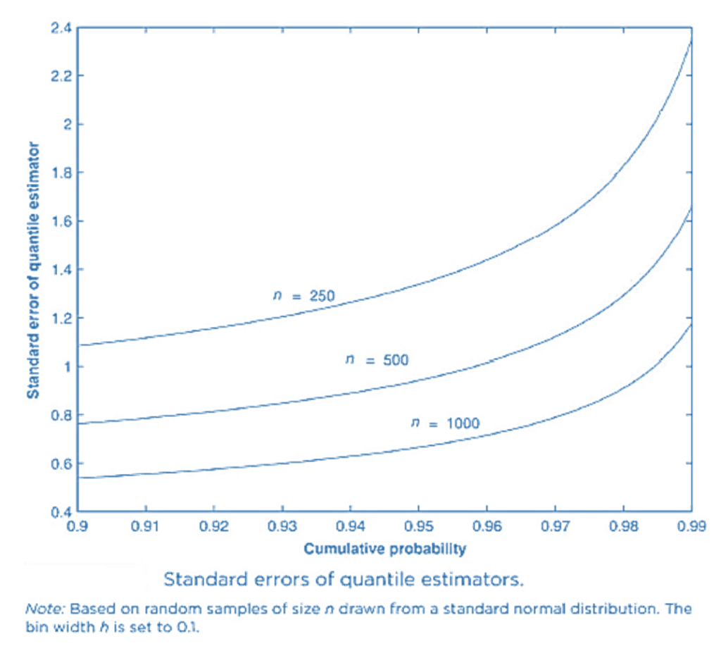
• The previous expression shows that the quantile standard error depends on p, the sample size n and the pdf value f(q). The way in which the (normal) quantile standard errors depend on these parameters is apparent from this figure.
• This shows that:
  • 1. The standard error falls as the sample size n rises.
    2. The standard error rises as the probabilities become more extreme and we move further into the tail-hence, the more extreme the quantile, the less precise its estimator.
  • In addition, the quantile standard error depends on the probability density function f(.)-so the choice of density function can make a difference to our estimates-and also on the bin width h, which is essentially arbitrary.
  • The standard error can be used to construct confidence intervals around our quantile estimates in the usual textbook way.
  • For example,
  • • a 90% confidence interval for a quantile q is given by

• • • a 95% confidence interval for a quantile q is given by

Also if we take a standard normal VaR at 95% confidence, (or in other words, 95% VaR of a standard normal), then q itself will be 1.645. So do not get confused. Remember VaR is one-tailed whereas confidence level is two tailed. So choose the values carefully.

•  
• Estimate the 90% confidence interval for a 95% VaR estimated on a sample of size of n = 1000 to be drawn from a standard normal distribution, based on an assumed bin width h = 0.1. Then use h = 0.2 and estimate it again.
• The quantile-standard-error approach is easy to implement and has some plausibility with large sample sizes. However, it also has weaknesses relative to other methods of assessing the precision of quantile (or VaR) estimators-it relies on asymptotic theory and requires large sample sizes; it can produce imprecise estimators, or wide confidence intervals; it depends on the arbitrary choice of bin width; and the symmetric confidence intervals it produces are misleading for extreme quantiles whose ‘true’ confidence intervals are asymmetric reflecting the increasing sparsity of extreme observations as we move further out into the tail.

QQ Plot Graphs

• It graphs the predicted quantile against the empirical quantile.
• QQ Plots (Quantile-Quantile plots) are plots of two quantiles against each other. A quantile is a fraction where certain values fall below that quantile. For example, the median is a quantile where 50% of the data fall below that point and 50% lie above it. The purpose of QQ plots is to find out if two sets of data come from the same distribution. A 45-degree angle is plotted on the QQ plot; if the two data sets come from a common distribution, the points will fall on that reference line.
  Source – https://www.statisticshowto.datasciencecentral.com/q-q-plots/