FRM Part 1 · Quantitative Analysis · Chapter QTA 7
Linear Regression
Learning Objectives
- Describe the models which can be estimated using linear regression and differentiate them from those which cannot.
- Interpret the results of an ordinary least squares (OLS) regression with a single explanatory variable.
- Describe the key assumptions of OLS parameter estimation.
- Describe the properties of OLS estimators and their sampling distributions.
- Construct, apply, and interpret hypothesis tests and confidence intervals for a single regression coefficient in a regression.
- Explain the steps needed to perform a hypothesis test in a linear regression.
- Describe the relationship among a t-statistic, its p-value, and a confidence interval.
- Estimate the correlation coefficient from the R² measure obtained in linear regressions with a single explanatory variable.
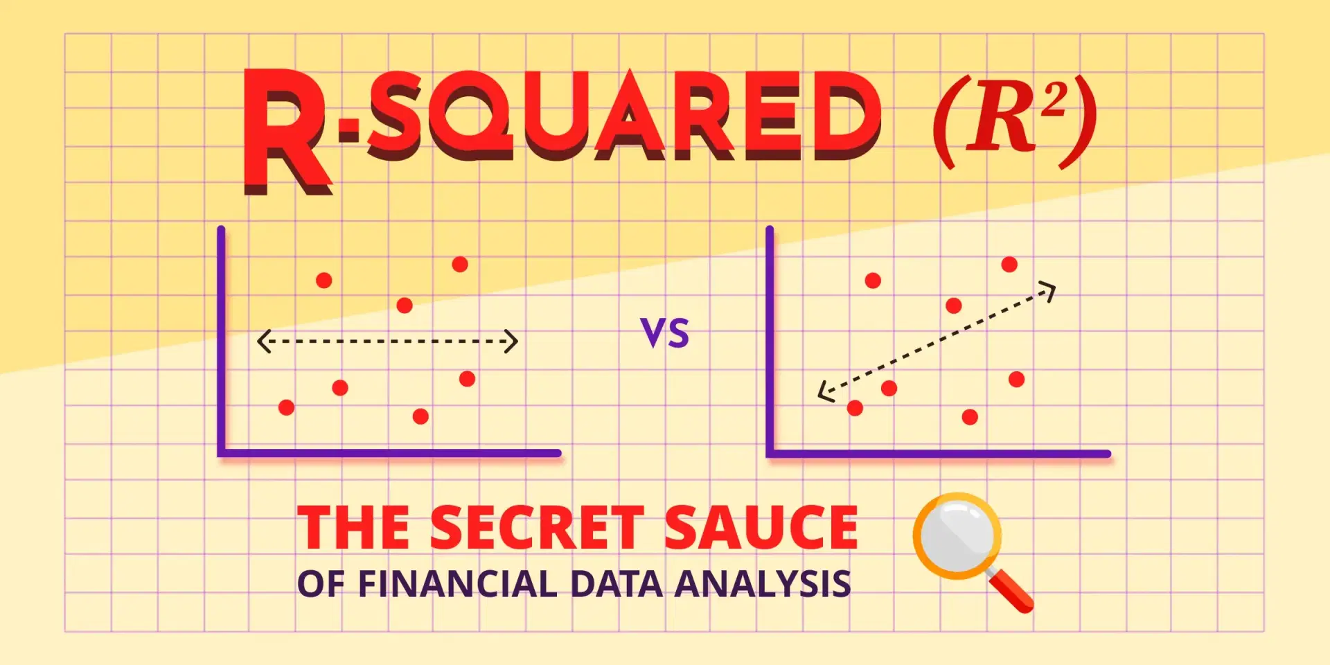
Correlation, from an earlier chapter, tells you that two variables move together, but it treats them as equals and stops there. Risk work usually needs more: how much does a stock move when the market moves one percent, how large a hedge cancels an exposure, how much of a fund’s return is skill rather than market beta. Answering those questions means fitting a line, and linear regression is the tool that fits it, quantifies it, and tests it.
Regression treats the two variables asymmetrically. One is the dependent variable, the thing being explained; the other is the explanatory variable, the thing doing the explaining, with causality assumed to run from explanatory to dependent. This chapter builds the single-explanatory-variable model from the ground up: the equation, the least-squares fit, the assumptions that make the fit trustworthy, the tests on the slope, and the three finance applications, market beta, the hedge ratio, and manager alpha, that are really the same regression wearing different labels.
Key Takeaways
- The model Y = α + βX + ε splits Y into a line, α + βX, and a mean-zero shock; β is the slope, α the intercept.
- Regression can estimate any model that is linear in its coefficients, including logarithms, polynomials, and dummies; it cannot estimate a parameter buried inside a nonlinear function.
- Ordinary least squares picks the line that minimizes the sum of squared residuals, giving β̂ = Cov(X, Y) / Var(X) and α̂ = Ȳ − β̂X̄.
- OLS is unbiased, consistent, and approximately normal in large samples when its assumptions hold, which is what licenses hypothesis tests.
- A coefficient’s t-statistic, p-value, and confidence interval always agree on significance, testing whether the coefficient differs from zero.
- R² is the fraction of variation explained; in a single-variable regression it equals the squared correlation, so the correlation is the signed square root of R².
The Linear Regression Model
The bivariate linear regression model writes the dependent variable as a straight-line function of one explanatory variable, plus a random shock.
where Y is the dependent variable, X the explanatory variable, α (alpha) the intercept, β (beta) the slope or regression coefficient, and ε (epsilon) the shock, or error, a mean-zero component of Y that X cannot explain.
Three names carry the meaning. The slope measures how sensitive Y is to X: the change in Y per one-unit change in X. The intercept is the level of Y when X is zero. The shock is everything else, the part of Y left unexplained; it is exactly the presence of this shock that makes the data scatter around the line rather than lie on it, and that is why the relationship must be estimated statistically rather than solved with algebra. Different fields rename these parts, calling Y the regressand or left-hand-side variable and X the regressor or right-hand-side variable, but the structure is always the same.
Which Models Can Be Estimated
The word “linear” in linear regression is easy to misread. It does not mean the relationship between the variables must be a straight line. It means the model must be linear in its coefficients: each term is a single unknown coefficient multiplied by a known variable, and the shocks are added on. Three requirements capture this, that the model be linear in the coefficients, that the error be additive, and that the variables be observable.
This is more permissive than it first appears, because the variables themselves may be transformed. A squared term, a logarithm, or a product of two variables can all serve as an explanatory variable, since each is a known quantity multiplied by a single coefficient. So polynomials, log-log models, dummy variables, and interactions are all fair game, and they let a curved relationship be captured within a linear regression.
where the left model is linear in the coefficients even though it is curved in X, so it can be estimated by setting a second explanatory variable equal to X squared. The right model cannot be estimated, because the unknown power γ (gamma) sits inside a nonlinear function and cannot be isolated as a coefficient times a variable.
The dividing line is where the unknown parameters live. If every unknown appears as a plain multiplier of an observable term, the model is estimable, however bent the curve. If an unknown is trapped inside a power, an exponent, or another nonlinear wrapper, it is not. Taking logarithms often rescues an otherwise non-estimable model: a multiplicative relationship with a coefficient in the exponent becomes additive and linear once both sides are logged.
Ordinary Least Squares
Ordinary least squares, or OLS, is the standard method for fitting the line. It chooses the intercept and slope that make the fitted line as close to the data as possible, where closeness is measured by the sum of squared vertical distances from the points to the line. The distances are squared so that positive and negative misses do not cancel, and so that large misses are penalized heavily. Minimizing that sum gives clean closed-form estimators.
where Cov(X, Y) is the sample covariance, Var(X) the sample variance of the explanatory variable, and X̄, Ȳ the two sample means. The slope is the covariance scaled by the variance of X; the intercept then forces the line through the point of averages.
The fitted values are the line’s predictions, and the residuals are what is left over, the vertical gaps between the actual points and the line. The residuals are the sample stand-in for the unobservable shocks, and the variance of the shocks is estimated by the sum of squared residuals divided by n minus 2, the minus 2 accounting for the two parameters, the slope and intercept, already estimated from the data. Figure 1 shows the fitted line through a scatter, with one residual marked.
A stock’s monthly excess return (Y) is regressed on the market’s excess return (X). The sample gives a covariance of Cov(X, Y) = 0.0054, a variance of X of Var(X) = 0.0036, and means of X̄ = 0.5% and Ȳ = 0.9%. Estimate the slope and intercept.
Step 1. The slope is the covariance over the variance of X.
Step 2. The intercept forces the line through the averages.
Answer: a slope of 1.5 and an intercept of 0.15% per month. The stock moves 1.5% for every 1% the market moves, so it is more volatile than the market, and it earns a small 0.15% a month beyond what its market exposure explains. Whether that 0.15% is real skill or just noise is a question for the hypothesis test later.
Interpreting the Slope and Intercept
Reading a regression output is a core skill, and the two coefficients answer different questions. The slope is a sensitivity: it says how much the dependent variable is expected to change when the explanatory variable rises by one unit, holding the shock at its mean of zero. A slope of 1.5 in the beta example means a one-percent market move is associated with a one-and-a-half-percent stock move.
The intercept needs more care. Literally, it is the value of Y when X is zero, but that reading is only meaningful when zero is a value X can actually take. If the explanatory variable is a firm’s market capitalization, which is always positive, the intercept describes a point outside the data and should not be interpreted as a real prediction. In the CAPM setting, though, a zero market excess return is perfectly possible, so the intercept there has a genuine meaning: the return earned when the market is flat.
Reading the intercept as a meaningful “starting value” when the explanatory variable can never be zero. If X ranges over firm sizes, interest rates far from zero, or any strictly positive quantity, the intercept is just the number that positions the line, not a forecast at X equal to zero. Interpret the intercept literally only when zero lies within, or realistically near, the range of the data.
The Key OLS Assumptions
OLS produces estimates from almost any data, but those estimates are only trustworthy, unbiased, consistent, and testable, when a set of assumptions holds. Exhibit 1 lists the key ones. The single indispensable one is that the explanatory variable actually varies; the rest secure the statistical properties that make inference valid.
| Assumption | What it requires | Why it matters |
|---|---|---|
| Variance of X > 0 | The explanatory variable takes more than one value | Without spread in X, no slope can be identified |
| Linear in coefficients | Each term is one coefficient times one variable | Makes the model estimable by OLS at all |
| Mean-zero shocks | The error has mean zero given X, carrying no information about X | Keeps the estimates unbiased |
| iid observations | Data are independent, identically distributed draws | Justifies the standard-error formulas |
| Homoskedasticity | The error variance is constant across X | Ensures the usual standard errors are correct |
| No large outliers | Extreme points are rare | Squared errors let one outlier distort the whole fit |
Two of these deserve a picture. Homoskedasticity means the scatter around the line is equally wide everywhere; when instead the scatter fans out as X grows, the errors are heteroskedastic, and the usual standard errors become unreliable even though the slope estimate itself stays sensible. Figure 2 contrasts the two. Real financial data are frequently heteroskedastic, which is why practitioners often adjust the standard errors rather than trust the textbook formula blindly.
Properties and Sampling Distributions
When the assumptions hold, the OLS estimators inherit exactly the good properties from the estimation chapter. They are unbiased, correct on average, so the expected slope equals the true slope. They are consistent, converging to the truth as the sample grows. And in large samples they are approximately normally distributed, which is what allows the slope to be tested with the familiar critical values.
where σ² is the variance of the shocks and σX² the variance of the explanatory variable. The variance of the slope estimate falls with the sample size n, falls when X is more spread out, and rises when the data are noisier.
The formula carries a practical lesson about what makes a slope precise. More data help, as always. Noisier data, a larger error variance, hurt. And crucially, a wider spread of the explanatory variable helps: it is far easier to pin down a slope when X ranges widely than when every observation crowds into a narrow band. This is why a regression estimated over a period when the market barely moved will have a poorly determined beta, however many observations it uses.
Testing a Regression Coefficient
The most common question about a regression is whether the slope is really different from zero, that is, whether X explains Y at all. This is an ordinary hypothesis test, applied to the coefficient. The test statistic is the estimated coefficient minus the null value, divided by its standard error, and under the null it is approximately standard normal.
where β0 is the null value, usually 0, and s.e.(β̂) is the standard error of the slope. The default t-statistic reported by software tests the null that the coefficient is 0, so a value above about 1.96 in absolute value signals significance at 5 percent.
The three ways of expressing the result, the t-statistic, the p-value, and the confidence interval, always agree, and the exam likes to check that a candidate knows this. The coefficient is significant at the 5 percent level exactly when the t-statistic exceeds 1.96 in magnitude, the p-value falls below 0.05, and the 95 percent confidence interval excludes the null value. Exhibit 2 shows a standard regression output row for the beta example, the format every statistics package produces.
| Coefficient | Estimate | Std. error | t-stat | p-value | 95% CI |
|---|---|---|---|---|---|
| Slope (β) | 1.50 | 0.30 | 5.00 | 0.000 | [0.91, 2.09] |
| Intercept (α) | 0.15% | 0.20% | 0.75 | 0.454 | [−0.24%, 0.54%] |
From Exhibit 2, decide whether the slope differs from zero, and whether the intercept (the alpha) is statistically significant, both at the 5% two-sided level.
Step 1. The slope. Its t-statistic is 5.00.
Step 2. The intercept. Its t-statistic is 0.75.
Answer: the slope is highly significant (t = 5.0, p ≈ 0, and its interval excludes zero), so the stock genuinely tracks the market. The alpha, though positive at 0.15%, has a t-statistic of only 0.75, a p-value of 0.45, and an interval that straddles zero, so it cannot be distinguished from luck. The stock has real market exposure but no proven skill.
R-Squared and the Correlation
Beyond the coefficients, a regression reports how well the line fits, summarized by R-squared. It is the fraction of the variation in the dependent variable that the model explains, running from 0, the line explains nothing, to 1, the line explains everything and the points lie exactly on it. A high R-squared means the explanatory variable accounts for most of the movement in the dependent variable; a low one means most of the movement is left in the shocks.
For a regression with a single explanatory variable there is a clean identity: R-squared equals the square of the sample correlation between the two variables. That gives a direct route back to the correlation coefficient, take the square root of R-squared, and attach the sign of the slope. It is the required skill of recovering a correlation from a reported R-squared. Figure 3 contrasts a high-R-squared fit, where the points hug the line, with a low-R-squared one, where they scatter loosely around it.
where the sign of the slope β̂ fixes the sign of the correlation, since R-squared alone is always positive and cannot reveal direction.
The beta regression reports an R² of 0.56, and the estimated slope is positive. Recover the correlation between the stock and the market.
Step 1. Take the square root of R², and apply the sign of the slope.
Answer: a correlation of about 0.75. The R² of 0.56 says the market explains 56% of the stock’s return variation, leaving 44% to stock-specific shocks. Because the slope is positive, the correlation is the positive root, 0.75. Had the slope been negative, the correlation would be minus 0.75.
Applications: Beta, Hedging, and Alpha
Three of the most common regressions in finance are the same single-variable model with different labels, all built by regressing a portfolio’s excess return on a benchmark’s. Exhibit 3 lines them up. In each, the slope and the intercept carry a distinct real-world meaning, and the R-squared judges how appropriate the benchmark is.
| Application | Slope (β) means | Intercept (α) means | R² means |
|---|---|---|---|
| Market beta (CAPM) | Sensitivity to the market; systematic risk | Abnormal return beyond market exposure | Share of risk explained by the market |
| Hedging | The optimal hedge ratio to cancel the exposure | Expected return of the hedged position | How completely the hedge removes the risk |
| Performance evaluation | Sensitivity to the style benchmark | Manager skill, or alpha | How well the benchmark fits the fund |
In the CAPM, the slope is the market beta, the portfolio’s systematic risk, and the intercept is its alpha, the return earned beyond what the market exposure justifies. A positive, significant alpha is the statistical signature of skill. In hedging, the same slope is read as the optimal hedge ratio: to neutralize a position’s exposure to a risk factor, hold an offsetting position of that size in the factor, and the hedged portfolio’s variance is minimized. In performance evaluation, a fund’s return is regressed on its style benchmark; a good benchmark has a beta near one and a high R-squared, meaning it captures the fund’s risks, and a positive alpha then signals genuine outperformance rather than mere market exposure.
Whenever a return is regressed on a benchmark, the slope is the exposure and the intercept is the excess. That single sentence unlocks all three applications: beta is exposure to the market, the hedge ratio is exposure to the factor being hedged, and alpha is the excess left over after the benchmark is accounted for. The R-squared always answers the same question, how much of the portfolio the benchmark explains, which is how you judge whether the benchmark was the right one to use.
A desk holds a 20 million dollar equity portfolio. Regressing the portfolio’s return on the return of an index futures contract gives a slope of 0.8, with a high R². How large a futures position hedges the portfolio, and what does the R² add?
Step 1. The slope is the optimal hedge ratio, so the futures position matches the slope times the exposure.
Answer: a short futures position of about 16 million dollars neutralizes the portfolio’s exposure to the index. The high R² matters because it says the index explains most of the portfolio’s movement, so the hedge will remove most of the risk; a low R² would warn that much of the portfolio’s variation comes from elsewhere and would survive the hedge.
Can the relationship Y = α + β ln(X) + ε be estimated by linear regression? What about Y = α · Xβ · ε with a positive error?
Show answer
The first can be estimated directly: ln(X) is just a known transformed variable multiplied by a single coefficient, so the model is linear in the coefficients even though it is curved in X. The second cannot be estimated as written, because the coefficient sits in the exponent and the error is multiplicative. But taking logarithms of both sides turns it into ln Y = ln α + β ln X + ln ε, which is linear in the coefficients and can then be estimated. Logging often rescues a non-estimable multiplicative model.
A regression of a stock on the market gives a slope of 0.8 with a standard error of 0.5, over 40 months. Is the stock’s beta significantly different from zero at the 5% level?
Show answer
The t-statistic is the estimate over its standard error: 0.8 / 0.5 = 1.6. Since 1.6 is below the critical value of 1.96, the null that the true beta is zero cannot be rejected at 5 percent. Despite an estimated beta of 0.8, the standard error is large relative to the estimate, so this sample cannot establish that the stock is linked to the market at all. A longer sample, or a market that moved more, would sharpen the estimate.
A single-variable regression reports an R² of 0.09 with a negative slope. What is the correlation between the two variables, and what does the R² say about the fit?
Show answer
The correlation is the signed square root of R²: the square root of 0.09 is 0.3, and because the slope is negative the correlation is minus 0.3. The R² of 0.09 means the explanatory variable accounts for only 9 percent of the variation in the dependent variable, so 91 percent is left unexplained. The relationship exists but is weak, and predictions from this line would carry large errors.
A fund’s return is regressed on its style benchmark. The beta is 0.98 with a high R², and the alpha is 3% per year with a t-statistic of 2.8. What can be concluded?
Show answer
The benchmark is well chosen: a beta near one and a high R² mean it captures the fund’s risk exposures closely. Against that benchmark, the alpha of 3% has a t-statistic of 2.8, above 1.96, so it is statistically significant. The fund has delivered a genuine 3% a year of outperformance that its benchmark exposure does not explain, which is evidence of manager skill rather than luck or hidden beta.
Chapter Summary
- The model Y = α + βX + ε explains a dependent variable with one explanatory variable plus a mean-zero shock; the slope is sensitivity, the intercept the level at X = 0.
- Linear regression estimates any model linear in its coefficients, including logs, polynomials, dummies, and interactions; it cannot estimate a parameter inside a nonlinear function, though logging often helps.
- OLS minimizes the sum of squared residuals, giving β̂ = Cov(X, Y)/Var(X) and α̂ = Ȳ − β̂X̄; the shock variance uses a divisor of n − 2.
- The intercept is interpretable only when X can be zero; otherwise it merely positions the line.
- Key OLS assumptions: variance in X, linearity in coefficients, mean-zero shocks, iid data, homoskedasticity, and no large outliers. When they hold, OLS is unbiased, consistent, and asymptotically normal.
- The slope estimate is more precise with more data, less noise, and a wider spread of X.
- A coefficient’s t-statistic, p-value, and confidence interval always agree: significant at 5 percent when |t| > 1.96, p < 0.05, and the interval excludes the null.
- R² is the fraction of variation explained; in a single-variable regression it equals the squared correlation, so Corr = sign(β̂) × √R².
- The same regression gives market beta and alpha (CAPM), the optimal hedge ratio (hedging), and manager alpha against a benchmark (performance evaluation).
Frequently Asked Questions
What does linear regression assume, and which models can it estimate?
Linear regression requires a model that is linear in its unknown coefficients, with an additive error and observable variables. It does not require the model to be a straight line in the variables themselves. Polynomials, logarithms, dummy variables, and interactions can all be estimated, because these are still linear in the coefficients even though they are nonlinear in the variables. A model cannot be estimated by linear regression when an unknown parameter sits inside a nonlinear function, such as a variable raised to an unknown power, because there is then no way to isolate a single coefficient times a single variable.
What do the slope and intercept of a regression mean?
The slope, or regression coefficient, is the estimated change in the dependent variable for a one-unit increase in the explanatory variable, so it measures sensitivity. The intercept is the estimated value of the dependent variable when the explanatory variable is zero. The intercept is only meaningful when zero is a value the explanatory variable can actually take; otherwise it is just the number that positions the fitted line and should not be interpreted literally.
What are the key assumptions of OLS estimation?
Beyond requiring that the explanatory variable actually varies, ordinary least squares relies on several assumptions for its estimates to be reliable: the model is linear in the coefficients; the error has mean zero given the explanatory variable, so the error carries no information about it; the observations are independent and identically distributed; the error has constant variance, called homoskedasticity; and there are no extreme outliers. When these hold, the OLS estimators are unbiased, consistent, and approximately normally distributed in large samples, which is what makes hypothesis testing valid.
How do the t-statistic, p-value, and confidence interval for a coefficient relate?
They are three views of the same test of whether a coefficient differs from a null value, usually zero. The t-statistic is the estimated coefficient minus the null value, divided by its standard error. The p-value converts that t-statistic into a probability of seeing something at least as extreme if the null were true. The confidence interval is the estimate plus and minus a critical value times the standard error. All three agree: the coefficient is significant at 5 percent when the t-statistic exceeds about 1.96 in absolute value, the p-value is below 0.05, and the confidence interval excludes the null value.
What does R-squared measure, and how does it relate to correlation?
R-squared is the fraction of the variation in the dependent variable that the regression explains, ranging from 0 for no explanatory power to 1 for a perfect fit. In a regression with a single explanatory variable, R-squared equals the square of the sample correlation between the two variables. So the correlation coefficient can be recovered as the square root of R-squared, taking the sign of the estimated slope: a positive slope means a positive correlation, a negative slope a negative one.
What is the difference between correlation and regression?
Correlation treats two variables symmetrically and measures only the strength and direction of their linear association, as a single number between minus one and plus one. Regression treats the variables asymmetrically, with a dependent variable explained by an explanatory variable, and it produces a slope and an intercept that describe how one responds to the other, along with a fitted line for prediction. Regression assumes a direction of causality from the explanatory variable to the dependent variable, whereas correlation makes no such assumption.
What are alpha, beta, and the hedge ratio in the CAPM regression?
When a portfolio’s excess return is regressed on the market’s excess return, the slope beta measures the portfolio’s sensitivity to the market, its systematic risk, and it is also the optimal hedge ratio, the position in the market needed to cancel that exposure. The intercept alpha measures the abnormal return, the part of the portfolio’s return not explained by its market exposure, so a positive and significant alpha is evidence of skill. R-squared then measures how much of the portfolio’s variation the market explains, which indicates how appropriate the market is as a benchmark.
Loading comments...
Add your Thoughts: